Model Exploration

Kedify Predictor can create a temporary JupyterLab workspace for one MetricPredictor. The workspace reads that resource’s stored metric history, so you can visualize several forecasting techniques against the same data, compare their errors, and experiment with Prophet parameters before changing the production model.

The supplied notebooks are exploratory: they do not ingest measurements, update the MetricPredictor, or publish a model. Prophet remains the model used by the MetricPredictor custom resource.

Prerequisites

Before starting, make sure that:

• Kedify Predictor is installed with a chart version that includes notebook support.
• Predictor uses PostgreSQL. Notebook deployment is not supported with the default SQLite metric store. Follow the external PostgreSQL setup if needed.
• A MetricPredictor already exists and has stored metric data. Several notebooks require at least 1,800 finite measurements by default. The predictive scaling example shows how to bootstrap a model with historical CSV data.
• You can annotate the MetricPredictor, inspect resources in the keda namespace, and port-forward a Service.

The commands below use a MetricPredictor named e-shop in the app namespace. Replace both values with your resource’s name and namespace.

The notebook server has no authentication

The generated JupyterLab server intentionally has no token or password. Its Service is a cluster-internal ClusterIP, but any workload or user that can reach it can execute notebook code. The notebook also receives credentials for the Predictor database. Enable it only for trusted users, restrict in-cluster access where needed, and keep the port-forward bound to 127.0.0.1.

1. Check the MetricPredictor

Confirm that the resource exists and is collecting data:

kubectl get metricpredictor e-shop -n app -o wide

The notebook is scoped automatically to this resource’s model name. You do not need to configure a database query or model identifier in JupyterLab.

2. Deploy the notebook

Add the kedify.io/notebook=true annotation:

kubectl annotate metricpredictor e-shop -n app \
  kedify.io/notebook=true --overwrite

The Predictor controller creates a one-replica Deployment and a ClusterIP Service in the keda namespace. For names of at most 63 characters, both resources are named <metricpredictor-name>-<metricpredictor-namespace>, which is e-shop-app in this example.

List all notebook resources and wait for this Deployment to become available:

kubectl get deployment,service -n keda \
  -l app.kubernetes.io/name=kedify-prophet-notebook

kubectl rollout status deployment/e-shop-app -n keda --timeout=2m

If the combined name exceeds Kubernetes’ 63-character limit, the controller truncates it and adds a hash suffix. Use the label-based listing above to find the generated name.

3. Port-forward JupyterLab

The Service is not exposed outside the cluster. Forward its default port to localhost:

kubectl port-forward -n keda --address 127.0.0.1 \
  service/e-shop-app 8888:8888

Leave this command running and open http://localhost:8888 in a browser. Start with 00-index.ipynb, then open a technique-specific notebook. Run its cells from top to bottom to load the selected model’s measurements, create a chronological training/test split, fit the technique, and visualize its held-out and future forecasts.

The workspace uses an emptyDir volume. Download any notebooks or results you want to keep before undeploying it.

4. Compare the included forecasting techniques

The notebook image ships with the following examples:

Notebook	Technique	What it demonstrates
01-simple-exponential-smoothing.ipynb	Simple Exponential Smoothing (SES)	Estimates a changing level using alpha. It is small and stable, but multi-step forecasts are flat because it does not model trend or seasonality.
02-double-exponential-smoothing.ipynb	Holt’s double exponential smoothing	Adds a local linear trend to the level using alpha and beta. It suits non-seasonal trends but extrapolates a straight line.
03-triple-exponential-smoothing.ipynb	Holt-Winters triple exponential smoothing	Adds a repeating seasonal component using alpha, beta, gamma, and a known seasonal period. It works best when the cycle and trend remain stable.
04-linear-regression.ipynb	Linear regression	Fits one global time-based slope. It is fast and easy to interpret, but does not capture cycles or changing trends without additional features.
05-moving-averages.ipynb	Recursive moving average	Evaluates short, fixed-window forecasts at rolling historical origins. It is a useful near-term baseline, but long recursive forecasts converge toward a constant.
06-arma-arima.ipynb	AR, MA, and ARIMA	Compares lagged values, lagged forecast errors, and differencing on the same holdout. These models can work well for stable short-term linear dependence, but require choosing p, d, and q and do not add seasonality unless extended.
07-dynamic-harmonic-regression.ipynb	Dynamic harmonic regression with ARIMA errors	Uses Fourier terms for daily and weekly cycles and ARIMA for residual dependence. It handles multiple long seasonalities efficiently, but requires fixed periods, Fourier orders, and ARIMA orders.
08-fft.ipynb	Fast Fourier Transform (FFT) spectral forecasting	Finds dominant frequencies, filters noise, aligns phase, and optionally extrapolates a trend. It is very fast for stable periodic signals, but does not model changepoints, holidays, or calibrated uncertainty.
09-prophet.ipynb	Prophet	Reuses the production model-building and evaluation logic to combine a flexible trend, changepoints, multiple seasonalities, country holidays, custom seasonality, and uncertainty intervals.

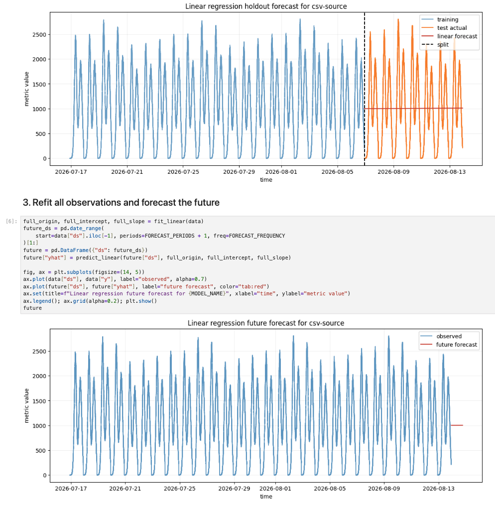
Notebook examples, from simple to complex

Linear regression reduces the history to one global trend. In this strongly seasonal example, its flat holdout and future forecasts make the model’s limitation immediately visible:

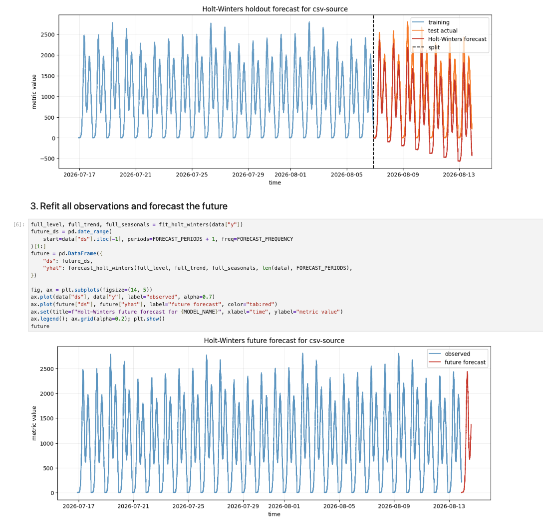
Triple exponential smoothing adds level, trend, and a repeating seasonal pattern. The Holt-Winters forecast follows the observed cycles, although its smoothing parameters and seasonal period still need careful tuning:

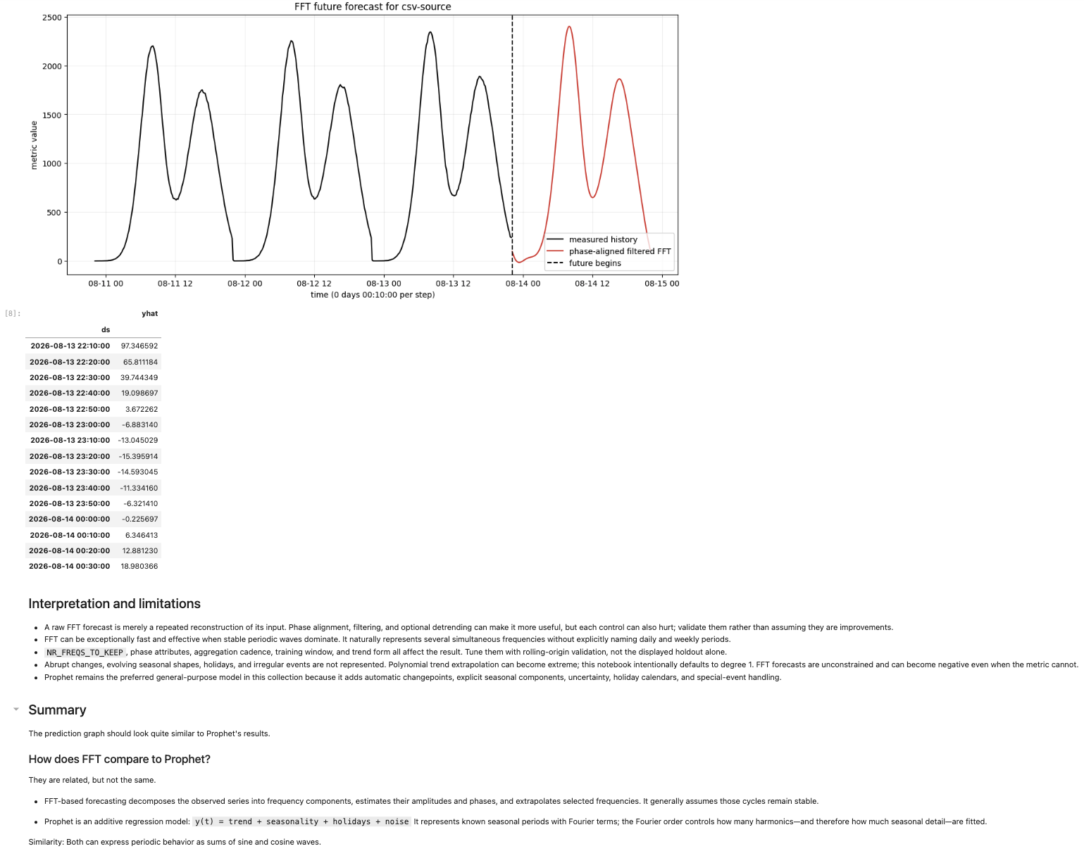
FFT forecasting decomposes the history into periodic components and extrapolates selected frequencies. Here, phase alignment carries the recurring pattern across the forecast boundary:

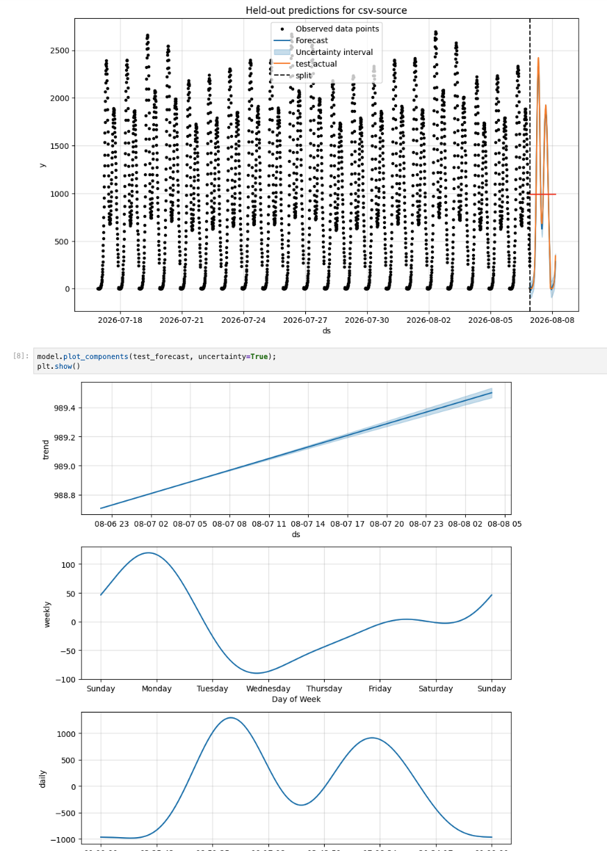
Prophet combines the forecast and uncertainty interval with explainable trend and seasonal components. The component plots help reveal what the model learned from the history:

Use the holdout metrics and forecast shape together when comparing techniques. A visually smooth in-sample fit is not evidence that a method predicts unseen data well.

5. Fine-tune Prophet

Open 09-prophet.ipynb. It initializes the experiment from the current MetricPredictor model settings and exposes editable values for:

• training/test split, look-back period, aggregation frequency, forecast frequency, and forecast periods;
• daily, weekly, and yearly seasonality;
• additive or multiplicative seasonality mode;
• changepoint prior scale;
• country holidays and holiday prior scale;
• custom seasonality name, period, and Fourier order; and
• the built-in six-hour seasonality and its Fourier order.

Change one group of parameters at a time, rerun the notebook, and compare the held-out MAPE, prediction graph, uncertainty interval, changepoints, and component plots. Aggregating dense measurements can keep interactive fitting within the notebook pod’s memory limit while retaining the broader history and seasonal structure.

Changes made in the notebook are isolated from the production model. When you find a better configuration, apply the corresponding values to .spec.model on the MetricPredictor and let Predictor retrain the model.

Optional notebook sizing

Notebook settings can be changed through Predictor Helm values. The defaults request 250m CPU and 512Mi memory and set a 2Gi memory limit:

notebook:
  port: 8888
  resources:
    requests:
      cpu: 250m
      memory: 512Mi
    limits:
      memory: 2Gi

Increase the memory limit if your experiments need a denser or longer training set. If you change notebook.port, use the same port on the right-hand side of the kubectl port-forward mapping.

Troubleshooting

• If no Deployment appears, run kubectl describe metricpredictor e-shop -n app and inspect its events. A MetricPredictorNotebookRequiresPostgres warning means Predictor is still configured for SQLite.
• If the pod reports missing model metadata or too few measurements, wait for the source to populate the Predictor database or bootstrap it with historical data.
• If the pod cannot start, inspect it with kubectl describe deployment/e-shop-app -n keda and kubectl get pods -n keda. The notebook image tag normally defaults to the Predictor chart application version with a -notebook suffix.

6. Undeploy the notebook

Stop the port-forward with Ctrl+C. After saving anything you need from the ephemeral workspace, remove the annotation:

kubectl annotate metricpredictor e-shop -n app kedify.io/notebook-

The Predictor controller then deletes the notebook Deployment and Service. Confirm that both are gone:

kubectl wait --for=delete deployment/e-shop-app -n keda --timeout=2m
kubectl wait --for=delete service/e-shop-app -n keda --timeout=2m